PROELL GOVERNOR

PROELL GOVERNOR

18.6.     Proell Governor

The Proell governor has the balls fixed at B and C to the extension of the links DF and EG, as

shown in Fig.The arms FP and GQ are pivoted at P and Q respectively.

Consider the equilibrium of the forces on one-half of the governor as shown in Fig. The instantaneous centre (I) lies on the intersection of the line PF produced and the line from D drawn perpendicualr to the spindle axis. The prependicular B M is drawn on ID.

PORTER GOVERNOR

18.5.     Porter Governor

The Porter governor is a modification of a Watt’s governor, with central load attached to the sleeve as shown in Fig. The load moves up and down the central spindle. This additional downward force increases the speed of revolution required to enable the balls to rise to any pre-determined level.

Consider the forces acting on one-half of the governor as shown in Fig.

Let	m  = Mass of each ball in kg,
	w  = Weight of each ball in newtons = m.g,
	M  = Mass of the central load in kg,
	W = Weight of the central load in newtons = M.g,
		r = Radius of rotation in metres,

h	=	Height of governor in metres ,
N  =		Speed of the balls in r.p.m .,
ω  =		Angular speed of the balls in rad/s
		= 2 π N/60 rad/s,
FC	=	Centrifugal force acting on the ball
		in newtons = m . ω 2.r,
T1	=	Force in the arm in newtons,
T2	=	Force in the link in newtons,

α = Angle of inclination of the arm (or upper link) to the vertical, and

=  Angle of inclination of the link

(or lower link) to the vertical.

Though there are several ways of determining the relation between the height of the governor (h) and the angular speed of the balls (ω), yet the following two methods are important from the subject point of view :

1.  Method  of  resolution  of  forces  ;  and  2.  Instantaneous centre method.

1. Method of resolution of forces

Considering the equilibrium of the forces acting at D, we have

T	cos β =		W	=	M . g
2			2			2
	T2	=	M . g
or
			2 cos			β

A big hydel generator. Governors are used to control the supply of working fluid (water in hydel generators).

Note : This picture is given as additional information and is not a direct example of the current chapter.

. . . (i)

Again, considering the equilibrium of the forces acting on B. The point B is in equilibrium

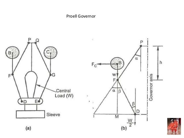
under the action of the following forces, as shown in Fig. 18.3 (b).
(i)	The weight of ball (w = m .g),
(ii)	The centrifugal force (FC),
(iii)	The tension in the arm (T1), and
(iv)	The tension in the link (T2).
Resolving the forces vertically,
	T1  cos α = T2	cos β + w =	M . g	+ m.g			. . . (ii)
		2
					T2	cos β =		M . g
				. . .  3
							2
Resolving the forces horizontally,
	T1 sin α + T2 sin β = FC

T1

sin α +

M . g

⋅ sin

β = FC

=

M .g

. . .  3 T2

2 cos

β

2 cos β

T

sin α +

M . g

⋅ tan

β = F

1

2

C

M . g

∴

T1  sin α = FC  –

⋅ tan β

. . . (iii)

2

Dividing equation (iii) by equation (ii),

T1  sin α

F   –

M . g

⋅ tan β

=

C

2

T1  cos α

M

. g

+ m . g

2

M . g

M

. g

			+ m . g	tan α = FC  –												⋅ tan β
	2				2

M . g

+ m . g

=

FC

–

M . g

⋅

tan β

2

tan α

2

tan α

Substituting

tan β

= q , and tan α =

r

, we have

tan α

h

M . g

+ m . g = m . ω2 . r ⋅

h

–

M . g

⋅ q

. . . (∴ F  = m.ω2.r)

2

r

2

C

m . ω2 . h = m . g +

M . g

(1 + q)

2

m +

M

(1 + q)

																								M . g														1										g
																																											2

∴

h

=

m . g

+

(1 + q)

=

⋅

														2												2							m						2
																			m .ω																						ω
. . . (iv)
																																				m +		M		(1 + q)
																			Mg										1																			g
2																															2

ω   =

m . g

+

(1 + q)

=

⋅

2

m . h

m

h

2 π N

2

m +

M

(1 + q)

g

=

2

⋅

m

h

60

m +

M

(1 + q )

2

m +

M

(1 + q)

g

60

895

∴

N

2

=

2

⋅

=

2

⋅

m

h

m

h

2π

. . . (v)

. . . (Taking g = 9.81 m/s²)

Notes : 1. When the length of arms are equal to the length of links and the points P and D lie on the same vertical line, then

tan α = tan β			orq =				tan α / tan β = 1
Therefore, the equation (v ) becomes
	N 2 =	( m + M )		⋅	895		. . . (vi)
					h
		m

2. When the loaded sleeve moves up and down the spindle, the frictional force acts on it in a direction opposite to that of the motion of sleeve.

If F = Frictional force acting on the sleeve in newtons, then the equations (v) and (vi) may be written as

M . g ±  F

m . g  +

(1

+ q )

N 2  =

2

⋅

895

. . . (vii)

m.g

h

= m . g + (M . g ± F ) ⋅

895

. . . (When q = 1) . . . (viii)

m . g

h

The + sign is used when the sleeve moves upwards or the governor speed increases and negative sign is used when the sleeve moves downwards or the governor speed decreases.

3. On comparing the equation (vi) with equation (ii) of Watt’s governor (Art. 18.5), we find that the m + M

mass of the central load (M) increases the height of governor in the ratio		.
	m

2.  Instantaneous centre method

In this method, equilibrium of the forces acting on the link BD are considered. The instantaneous centre I lies at the point of intersection of PB produced and a line through D perpendicular to the spindle axis, as shown in Fig. 18.4. Taking moments about the point I,

F  ⋅ BM  = w ⋅ IM  +

W

⋅ ID

C

2

= m .g ⋅ IM  +

M . g

⋅ ID

2

∴

FC

= m .g ⋅

IM

+

M . g

⋅

ID

BM

BM

2

= m .g ⋅

IM

+

M . g

IM  + MD

BM

2

BM

= m . g ⋅

IM

+

M . g

IM

+

MD

BM

2

BM

BM

= m . g tan α + ^{M . g} (tan α + tan β) 2

Fig. 18.4. Instantaneous centre method.

IM

MD

. . .  3

= tan α, and

= tan β

BM

BM

Dividing throughout by tan α,

FC

= m . g +

M . g

+

tan β

= m . g +

M . g

+ q)

=

tan β

1

(1

. . .  3q

tan α

2

tan α

2

tan α

We know that F  =  m.ω2.r,

and

tan α =

r

C

h

∴  m.ω2 . r ⋅

h

= m . g +

M .g

(1+ q)

r

2

m . g +

M . g

(1 + q )

m +

M

(1 + q)

1

g

or

2

2

h =

m

⋅ ω2  =

⋅ ω2

m

. . (Same as before)

When   tan α = tan β  or  q = 1, then

h =

m + M

⋅

g

ω2

m